DEMOCRATIZING SCIENTIFIC COMPUTING

Democratizing Modeling and Simulation and Scientific Computing
in the Era of Generative AI

Opportunities to develop custom code and UI to make scientific computing part of every workflow to accelerate scientific discovery, technology innovation and commercialization, and unparalleled process, energy, and material efficiency

Dr. Sreekanth Pannala

The Exponential Engine

Computing power has grown exponentially, democratizing access to computational resources

Compute Power (FLOPS)

Cost per GFLOP

Memory & Storage

10⁹×
Compute Growth
Since 1960s
10⁷×
Cost Reduction
Per GFLOP
10⁶×
Storage Growth
Since 1980s
10⁵×
Network Speed
Dial-up to Fiber

The New Computing Paradigm

From specialized monoliths to democratized, purpose-driven tools

Old Paradigm

  • Monolithic codes — Large, complex software requiring years to master
  • Specialized training — Steep learning curves limit accessibility
  • Siloed workflows — Disconnect between experiments and computation
  • Expert-only — Computing power locked behind technical barriers

New Paradigm

  • Purpose-driven code — AI-generated tools tailored to specific workflows
  • Intuitive UI/UX — Accessible interfaces hide complexity, enable rapid iteration
  • Closed-loop integration — Experiments ↔ Data ↔ Simulations in continuous cycle
  • Democratized access — Everyone participates in computational discovery

Closed-Loop Innovation Cycle

DEMOCRATIZE
Experiments
Data
AI Code
Simulation

The Opportunity: Complex Fluidized Beds

Constructing models faster than real-time, trained against actual data and detailed computational data

The Challenge

  • Industrial Scale: Fluidized bed reactors handle billions of particles in complex flow patterns
  • Real-time Need: Operators need predictions faster than the process itself
  • Multi-source Data: Combine experimental measurements with high-fidelity simulations

The Solution

  • AI-Accelerated Models: Reduced-order models trained on CFD-DEM data run 1000× faster
  • Continuous Learning: Models update as new experimental data becomes available
  • Accessible UI: Operators use simple interfaces without needing CFD expertise

Result: Real-time digital twins that democratize complex reactor modeling across the organization

The Multiphase Dilemma

Commercial reactors contain billions of particles. Tracking them all (Euler-Lagrange) is computationally impossible. Averaging them (Euler-Euler) loses the physics.

Multiscale & Multiphysics Nature

Phenomena spanning 10+ orders of magnitude in time and space
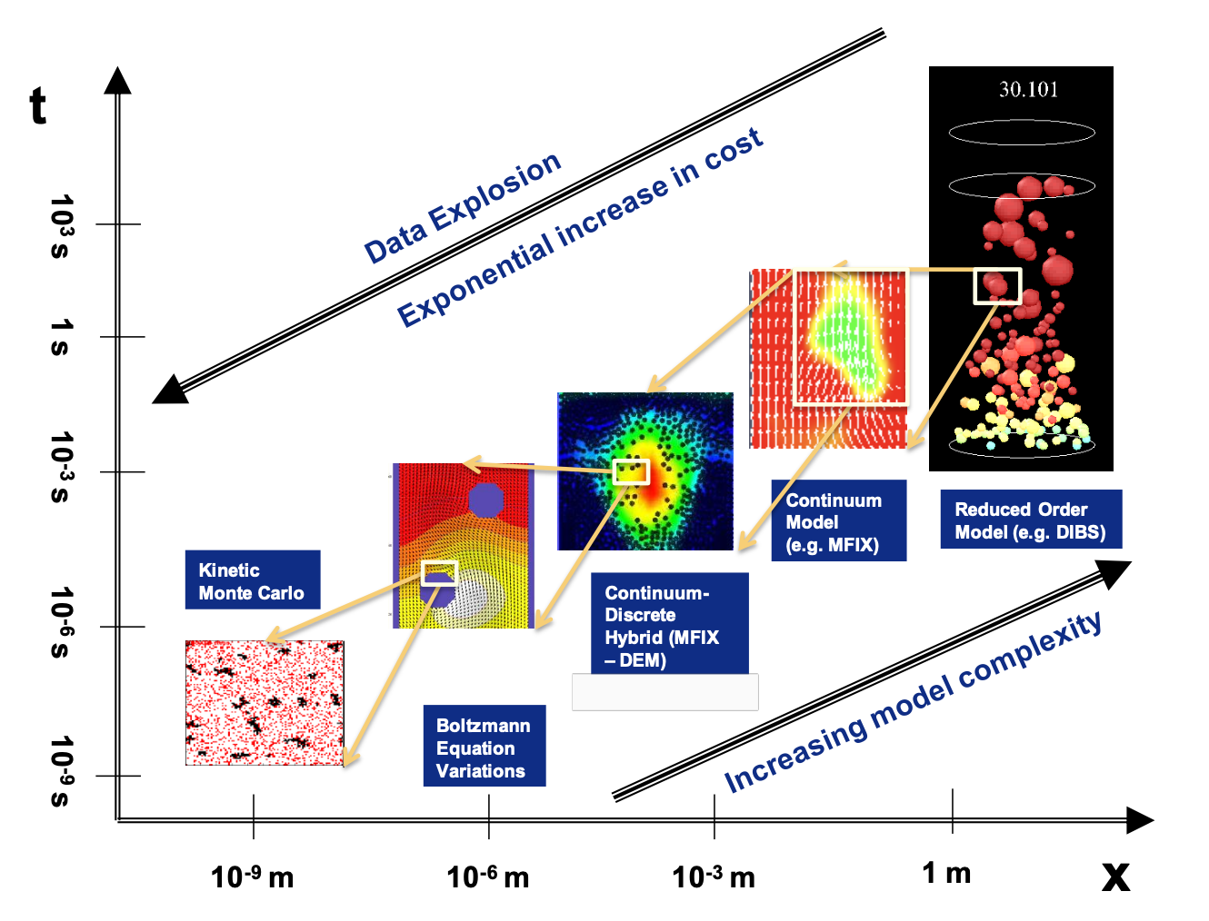
Multiscale multiphysics illustration
From molecular interactions to reactor-scale flows

Too Slow (DNS/DEM)

Direct Numerical Simulation tracks every particle and resolves all scales.

10⁹+ particles → Years of CPU time for seconds of real time

Too Vague (TFM)

Two-Fluid Model averages out all structure using empirical closures.

Constitutive relations → Loses mesoscale structures (clusters, bubbles)

Just Right (DIBS/DHRDM)

Agent-based approach tracks mesoscale structures (bubbles, clusters) directly.

10³-10⁴ agents → Fast, accurate, captures emergent phenomena

Agent-Based Approach

Instead of tracking particles, we track Bubbles as discrete agents.

// 1. Lagrangian Tracking
dx/dt = V_bubble (position independent of grid)
// 2. Wake Effect (Interaction)
if (in_wake(neighbor)) { accel += 0.05; move_to_center(); }
// 3. Coalescence
if (touching(neighbor)) { merge_volumes(); }
A
B

Bubble A accelerates into B's wake

DIBS Control Panel

Adjust parameters

Simulation

Time: 0.00 s

Bubbles: 0

Bed Height: 50.0%

Bed & Flow

Bubble Formation

Solids Conservation: Bubbles rise through solids. When bubbles reach freeboard (no solids), they merge into gas phase. Total solids volume is conserved.

Pannala et al., Chaos (2004); Int. J. Chem. React. Eng. (2003)

The "Drag Crisis"

Reality (Fine Scale)

Gas flows AROUND dense clusters.
Net Drag = LOW

Simulation (Coarse Grid)

Uniform Average

Model sees uniform "soup".
Net Drag = HIGH (Incorrect)

THE ALGORITHM

Dynamic Heterogeneity-Resolving Drag Model

We use DBSCAN (Density-Based Spatial Clustering) to identify clusters on the fly during the simulation.

  1. Detect: Scan grid for regions where density > φcrit.
  2. Cluster: Group contiguous dense cells using DBSCAN (minPts, epsilon).
  3. Correct: Apply different drag laws to "Cluster" cells vs "Dilute" cells.
// Pseudocode for DHRDM Step
for cell in grid:
if cell.density > phi_crit:
candidates.push(cell)

clusters = DBSCAN(candidates, eps=1.5, minPts=3)

for cell in grid:
if cell in clusters:
drag = drag_cluster(cell) // LOW
else:
drag = drag_standard(cell) // HIGH

Riser Lab

Cluster Threshold (φ) 0.20
Search Radius (ε) 1.5
Solids Holdup
0.00
Dilute
Dense
Cluster

Calibrating DHRDM from Experimental Data

Using NETL riser footage and image analysis to extract cluster statistics

1

Capture Video

High-speed camera records NETL pilot-scale riser (1m height, 800×588px, 15 fps)

Source Data:
  • • Duration: 84 seconds
  • • Resolution: 1.7 mm/pixel
  • • Sample rate: 1 frame/sec
2

Image Processing

Adaptive thresholding + morphological operations reveal cluster boundaries

mask = threshold(frame)
mask = closing(mask)
labels = DBSCAN(mask)
3

Extract Statistics

Measure cluster properties to calibrate DHRDM parameters

Measured Properties:
  • • Mean width: 6.6 mm
  • • Mean height: 91 mm
  • • Avg clusters/frame: 84

Raw NETL Video

NETL pilot-scale riser showing particle clusters

Binary Segmentation

Binary mask showing dense regions

Adaptive threshold isolates dense regions

Cluster Labels (DBSCAN)

DBSCAN cluster overlay

DBSCAN identifies clusters → calibrates φcrit, ε, minPts

Result: Experimental cluster statistics set realistic targets for simulation parameters

THE VISION

Reimagine Scientific Workflows

Simple models trained on rich datasets and made widely accessible can revolutionize scientific and process workflows

Democratizing modeling and simulation and scientific computing in the era of Generative AI creates unprecedented opportunities to develop custom code and UI, making scientific computing part of every workflow to accelerate scientific discovery, technology innovation and commercialization, and achieve unparalleled process, energy, and material efficiency

Accelerate Discovery

From years to months, from months to days

Enable Innovation

Everyone becomes a computational scientist

Maximize Efficiency

Process, energy, materials optimized in real-time

Dr. Sreekanth Pannala

Thank you

APPENDIX

TSDaw

Chaos and Time Series Analysis Toolkit

About TSDaw

A Python-based nonlinear dynamics and chaos theory analysis package inspired by TISEAN. TSDaw provides modern, modular implementations with both programmatic APIs and interactive web interfaces for analyzing chaotic and complex time series data.

Dedicated to C. Stuart Daw, educator and mentor in chaos theory

Open Source Repository

https://github.com/pannalas/TSDaw

MIT License • Python 96.7%

17 Core Modules

Comprehensive chaos theory algorithms

Web Interfaces

Streamlit UI & FastAPI endpoints

Production Ready

Docker support for deployment

Author: Sreekanth Pannala (with assistance from Generative AI tools)
Dedicated to former colleague, mentor, and friend, C. Stuart Daw

APPENDIX

TSDaw: Core Analysis Methods

Nonlinear Dynamics

  • AMI & FNN: Optimal delay and embedding dimension
  • Grassberger-Procaccia: Correlation dimension (D₂)
  • Lyapunov Exponents: Chaos quantification (Rosenstein)
  • Entropy Measures: Sample & permutation entropy

Recurrence & Fractal

  • RQA: Recurrence plots with RR, DET, LAM metrics
  • DFA: Detrended fluctuation analysis
  • Hurst Exponent: Long-range correlations
  • S-test: Attractor comparison (van Ommen)

Spectral Analysis

  • PSD: Welch, periodogram, spectrogram methods
  • Wavelet Analysis: Time-frequency decomposition
  • Multiple Windows: Hann, Hamming, Blackman, etc.

Symbolic & Testing

  • SAX Pipeline: Symbolic aggregate approximation
  • Surrogates: AAFT/IAAFT for nonlinearity testing
  • Prediction: Local linear k-NN forecasting
APPENDIX

TSDaw: Technologies & Architecture

Core Stack

Python 3.11+
NumPy ≥1.23
SciPy ≥1.10
Pandas ≥2.0
scikit-learn ≥1.3

Web Frameworks

FastAPI REST API
Streamlit Interactive UI
Uvicorn ASGI Server
Pydantic Validation
HTMX Dashboard

Architecture Overview

Core Module

17 Python files implementing chaos theory algorithms

API Layer

FastAPI endpoints with Pydantic schemas

Frontend

Streamlit & HTMX interfaces

Test Coverage

pytest + pytest-cov

Deployment

Docker Ready

APPENDIX

TSDaw: Applications & Use Cases

Physiology

  • Heart rate variability analysis
  • EEG/ECG signal processing
  • Biological rhythm detection

Finance

  • Market dynamics analysis
  • Volatility and regime detection
  • Risk assessment patterns

Geophysics

  • Climate pattern analysis
  • Earthquake prediction models
  • Environmental monitoring

Engineering

  • System monitoring & control
  • Fault detection & diagnosis
  • Process optimization

Key Analytical Workflows

Parameter Estimation

Determine optimal embedding parameters before attractor reconstruction

Nonlinearity Testing

Validate presence of nonlinear dynamics vs. stochastic noise

Chaos Quantification

Measure sensitivity to initial conditions and fractal dimensions

Regime Detection

Identify transitions and drift in system behavior patterns